Charging GPU energy to the code that spent it

I spent the summer of 2025 at Oak Ridge on one question: does the fastest way to compute something also cost the least energy? A profiler ranks code by time, but clusters increasingly run under a power cap rather than a clock-rate target, so energy-to-solution is becoming the number that matters, and almost nothing in a normal HPC workflow reports it per region. So I built a tool that does, as a Kokkos Tools connector that attributes joules to each profiled region without touching the application it measures.

Start with the DBSCAN comparison from the poster, recomputed in September 2026 from the raw traces. ArborX ships two DBSCAN implementations, fdbscan and fdbscan-dense. On the same input and the same NVIDIA H100 NVL they return the same clusters, and over 64 runs of each, the dense one is faster and cheaper:

Medians over 64 runs of each variant.

variant	DBSCAN region	energy	mean power
fdbscan	2.69 s	777 J	288 W
fdbscan-dense	2.19 s	580 J	262 W

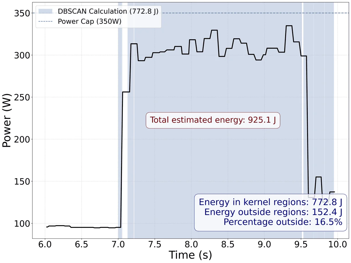
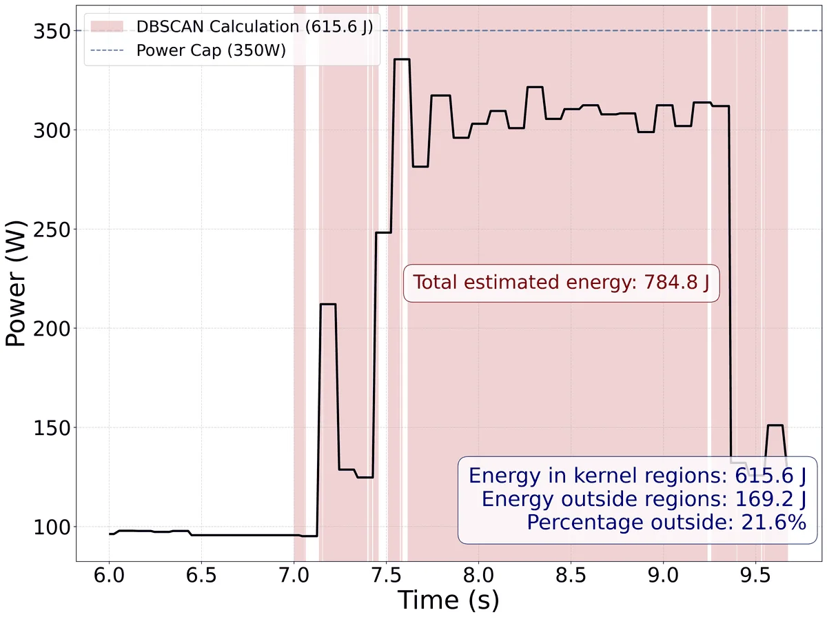
The poster presented the two runtimes as equal; the region timestamps show the 19% gap in the table. The traces of all 128 runs and the script that recomputes these figures are published with the poster, and a note at the end explains why the poster’s energy figures differ from the table’s.

One more thing the medians hide. The first 16 fdbscan-dense runs, consecutive at the start of the series, are about 1.5 times slower in every phase (3.4 to 3.9 s) and draw less power (222 W on average), which looks like a different machine state rather than the algorithm. I kept them in the medians. Without them the comparison barely moves (19% less time, 26% less energy); with them, the means over all 64 runs give 5% less time and 18% less energy. A bootstrap over the runs puts the median reductions at 17.6 to 19.3% for time and 24.9 to 26.0% for energy.

So the faster variant also wins on energy, but by more: 25% less energy for 19% less time, because its mean power is also 9% lower while it runs. A time profile would report the 19%; the extra 6 percentage points of energy only show up when you measure energy instead of inferring it from time.

Instrumentation you do not have to compile in

Kokkos already announces what it is doing. Every parallel_for, parallel_reduce and parallel_scan fires a begin callback before it launches and an end callback after it finishes, and you can wrap arbitrary spans in named regions with push and pop markers. A Kokkos Tools connector is just a shared library that implements those callbacks, and you attach it by pointing an environment variable at it: no recompile, no change to the application’s source. You set KOKKOS_TOOLS_LIBS to the path of the library and the runtime loads it.

So I could take a solver I did not write, that nobody wanted me to patch, and measure the energy of its regions by loading one extra library next to it. The connector listens to the events Kokkos is already emitting, and the measurement rides along.

You cannot read energy, only watch power

The obvious first version reads the power sensor at the begin callback, reads it again at the end, and multiplies the average by the duration; that is what the existing Variorum connector in Kokkos Tools does. It does not work, and the reason it does not work is the heart of the problem. NVIDIA’s management library, NVML, exposes nvmlDeviceGetPowerUsage, which returns the board’s instantaneous power draw in milliwatts. The catch is twofold. That value is refreshed only every 100 ms, and it averages just the last 25 ms of each interval (Yang, Adamek and Armour, SC24), so most of what the board does is never observed at all. Many kernels finish in far less than those 100 ms: begin and end frequently return the same stale reading, and the duration tells you nothing. And even when a region is long enough to span several updates, two point readings cannot describe a curve that rises and falls across it.

The deeper issue is that power is the wrong quantity to sample at the boundaries. Power is a rate, in watts. What you pay for is energy, in joules, and energy is the integral of power over time. Two readings give you two heights of a curve. The bill is the area under it. My first version reported nonsense on short kernels, sometimes zero, sometimes the power of the previous kernel, depending on which side of a sensor update the two readings landed, and that was the signal to stop sampling on the kernel’s schedule and start sampling on the clock’s.

A side thread, a fixed cadence, and a trapezoid

So sampling has to be separated from the kernels entirely. A background thread polls the power sensor on a fixed interval, every 20 ms in the current connector, and timestamps every reading, building a continuous trace of how the board’s draw moved through the whole run. The begin and end callbacks no longer read power at all. They record a wall-clock window, the moment the region opened and the moment it closed. To get a region’s energy, the connector integrates the power trace over that window with the trapezoidal rule, summing the little trapezoids between consecutive samples that fall inside it. Because the same region is entered many times, its joules accumulate across every call.

Sampling on the clock instead of on the kernel gives a continuous trace, but it cannot beat the sensor. With a 25 ms window every 100 ms, a single short kernel is effectively invisible, and adding up many launches does not fix a blind spot that recurs at the same phase. What the trace does measure reliably is a region much longer than the refresh interval: a solver phase, or a whole algorithm, like the two DBSCAN runs above. The poster pushes resolution a little further by repeating a run 64 times, shifting its start by 5 ms each time and keeping the highest reading per kernel. Those are the same 64 runs behind the medians above, where each run is integrated on its own. Either way the conclusion stands: per-kernel energy is out of reach through NVML.

The limits of the number

NVML reports power for the whole board, not per streaming multiprocessor, so this is whole-GPU attribution. If two kernels run concurrently on the same device, on separate streams, the trace cannot tell you which one drew which watt, and the energy of the overlap cannot be split cleanly between them. The total also includes whatever the board draws between regions: in the DBSCAN runs above, 16.5% and 21.6% of the energy falls outside any Kokkos region, which is why the 2025 connector reports both numbers. Whole-device attribution is enough to compare algorithms by energy, and not enough to rank individual kernels.

Two backends, two different questions

NVML answers one question: what this NVIDIA GPU drew. It reports per board, in milliwatts, NVIDIA only, and sees nothing outside the card. So the 2025 tooling has a second measurement tool built on Variorum (#302, beside the NVML one in #301), which is vendor-neutral and reads power at the node and socket level, including the CPU (through RAPL, the power counters built into Intel and AMD processors), the DRAM, and some non-NVIDIA GPUs. NVML gives you what the GPU drew, Variorum what the whole node drew. A region that looks cheap on the card can still be shuffling enough data to light up the CPU and the memory controllers around it, and only the node-level view catches that. You reach for NVML when the question is what the GPU itself spent, and for Variorum when you want the energy bill the machine room actually sees.

What per-region joules buy you

Once energy is attributed to the region that spent it, you can finally optimize the quantity you are actually billed for instead of using time as a stand-in and hoping the two agree. They need not agree: going fast can mean running the silicon at its power ceiling, and a slower memory-bound phase can be the cheaper one to run a million times. On DBSCAN they agree on the winner and differ on the margin: the energy gap (25%) is wider than the time gap (19%).

The sampling daemon I started was merged into kokkos/kokkos-tools (#300) in March 2026, after my ORNL mentor reworked it through review; the core (#299) and the NVML and Variorum connectors (#301, #302) are still open. The CSV trace first fed a Grafana and PostgreSQL dashboard; it now goes to energy-dashboard-for-kokkos, a single Rust binary with no daemon and no Docker, which prints a per-region energy table, exports a Perfetto timeline, and writes a standalone HTML report. The full results are on the page of the poster I co-authored with Daniel Arndt, Jakob Bludau and Damien Lebrun-Grandié (SMC 2025). What is still missing is resolution finer than the whole board and than the 100 ms refresh: attribution stays at the scale of the GPU, and I have no clean answer for concurrent streams.

Note on the figures. Four numbers describe fdbscan, and they measure different things. The table gives 777 J, the median over 64 runs of the DBSCANCalculation region alone. One of those runs, drawn on this site’s home page, spends 769 J in that region. The poster’s box, labeled DBSCAN Calculation, reads 772.8 J because it sums every kernel region of the run, and its 925.1 J total also counts the time outside any region.